How to Freeze a Row or Column in Google Sheets : Easy Guide
Google Sheets is a powerful and user-friendly spreadsheet tool that offers various features to enhance data organization and visualization. One of its most practical features is the ability to freeze rows or columns, ensuring that important headers or data remain visible as you scroll through your sheet. In this blog, we’ll walk you through how to freeze a row in Google Sheets, whether it’s the top row or a specific one, and even how to manage freezing rows in the Google Sheets app.
If you're looking to freeze rows or columns in Excel instead, follow the guide here.
Freezing rows is particularly helpful when working with large datasets. By freezing a row, you can:
- Keep headers visible for easy reference.
- Maintain context as you scroll through data.
- Improve overall navigation and usability of your spreadsheet.
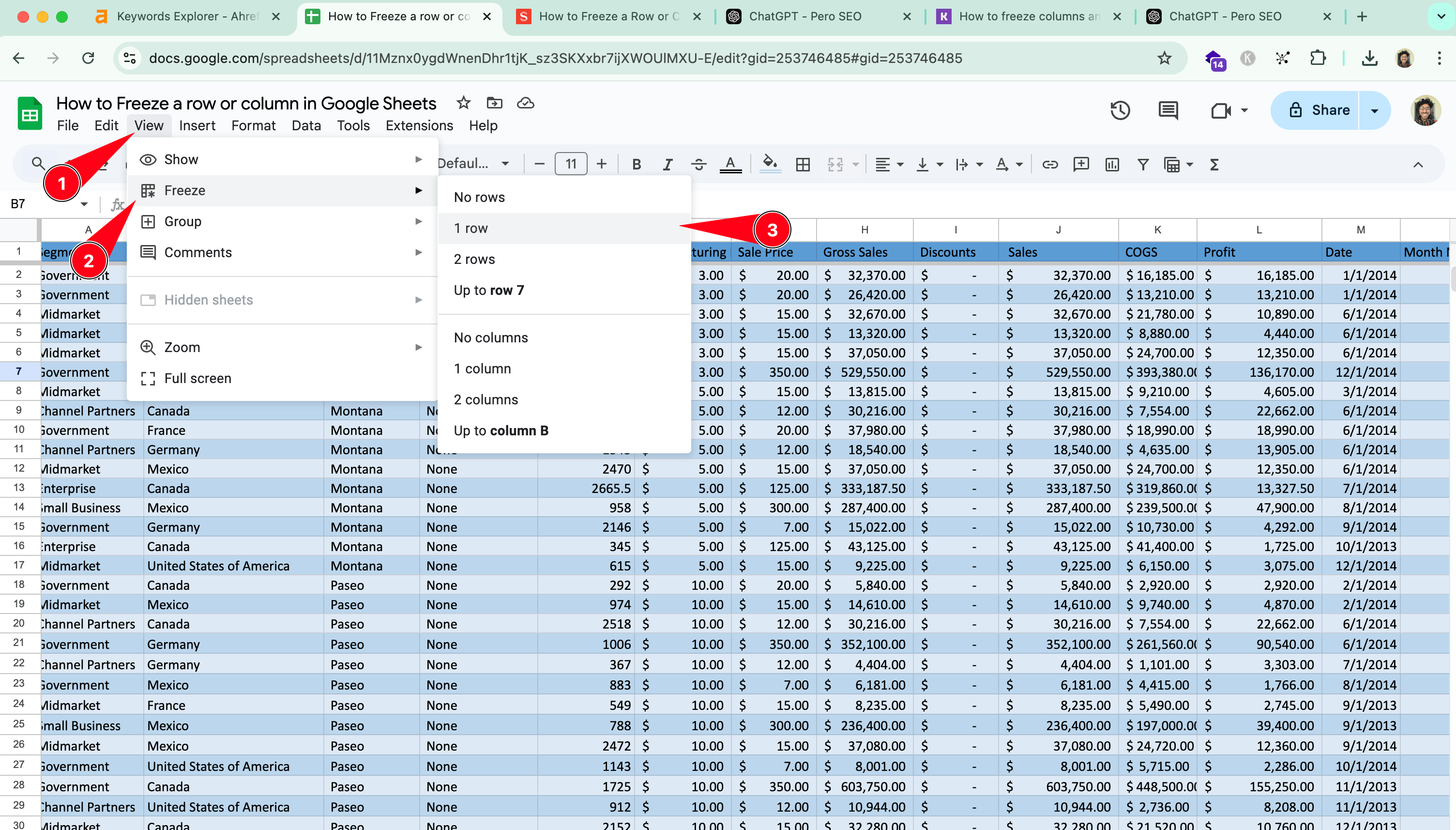
Freezing the top row is a common need, especially for spreadsheets with column headers. Follow these steps to freeze the top row:
- Open your Google Sheet:
- Navigate to the Google Sheet you want to edit.
- Go to the View Menu:
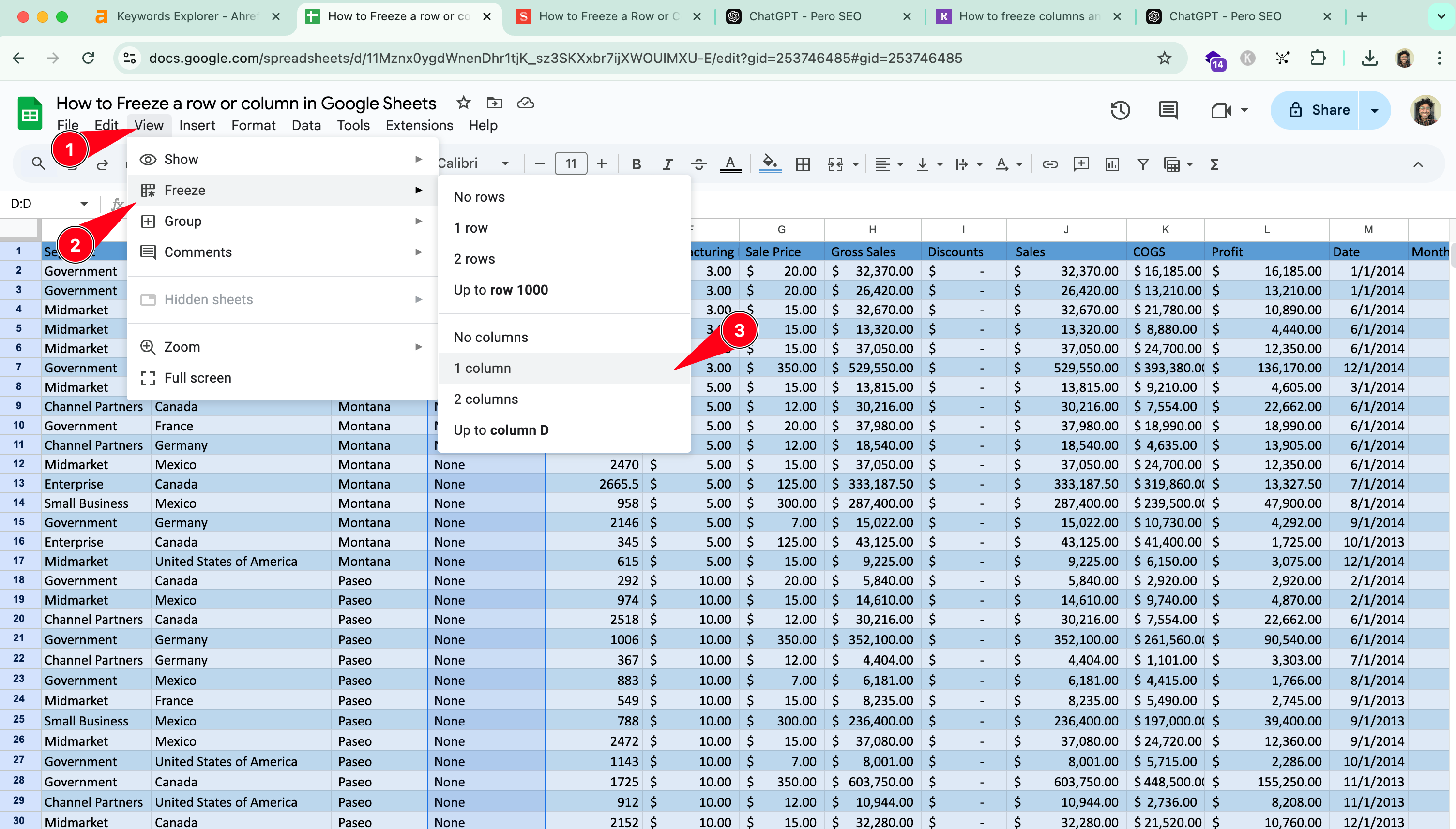
- Click on
Viewin the top menu.
- Click on
- Select Freeze > 1 Row:
- Hover over the
Freezeoption and select1 rowfrom the submenu.
- Hover over the
That’s it! Your top row is now frozen and will remain visible as you scroll down.
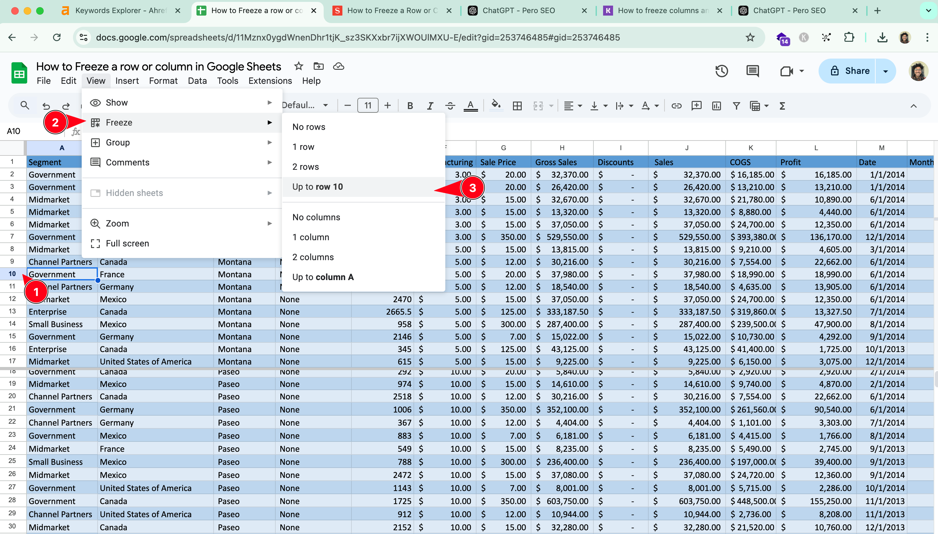
If you need to freeze a row other than the top row, here’s what you do:
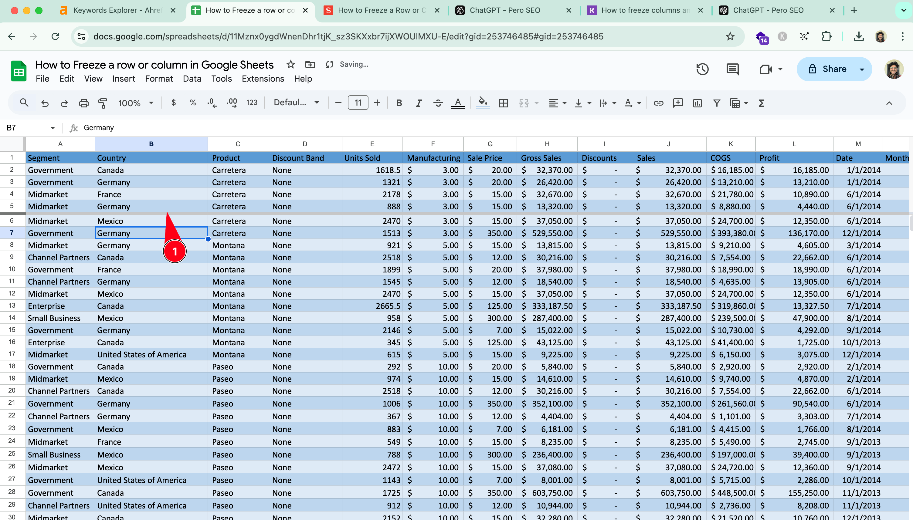
- Click the Row Number:
- Locate the row you want to freeze and click on its row number on the left-hand side.
- Drag the Freeze Line:
- Hover your cursor over the thick gray bar between the rows and drag it down to the desired row.
- Use the View Menu:
- Alternatively, go to
View > Freezeand select the number of rows you want to freeze. For example, if you want to freeze rows 1-3, chooseUp to row 3.
- Alternatively, go to
Freezing rows in the Google Sheets app on your mobile device is just as simple. The same method works on both Android and iOS.
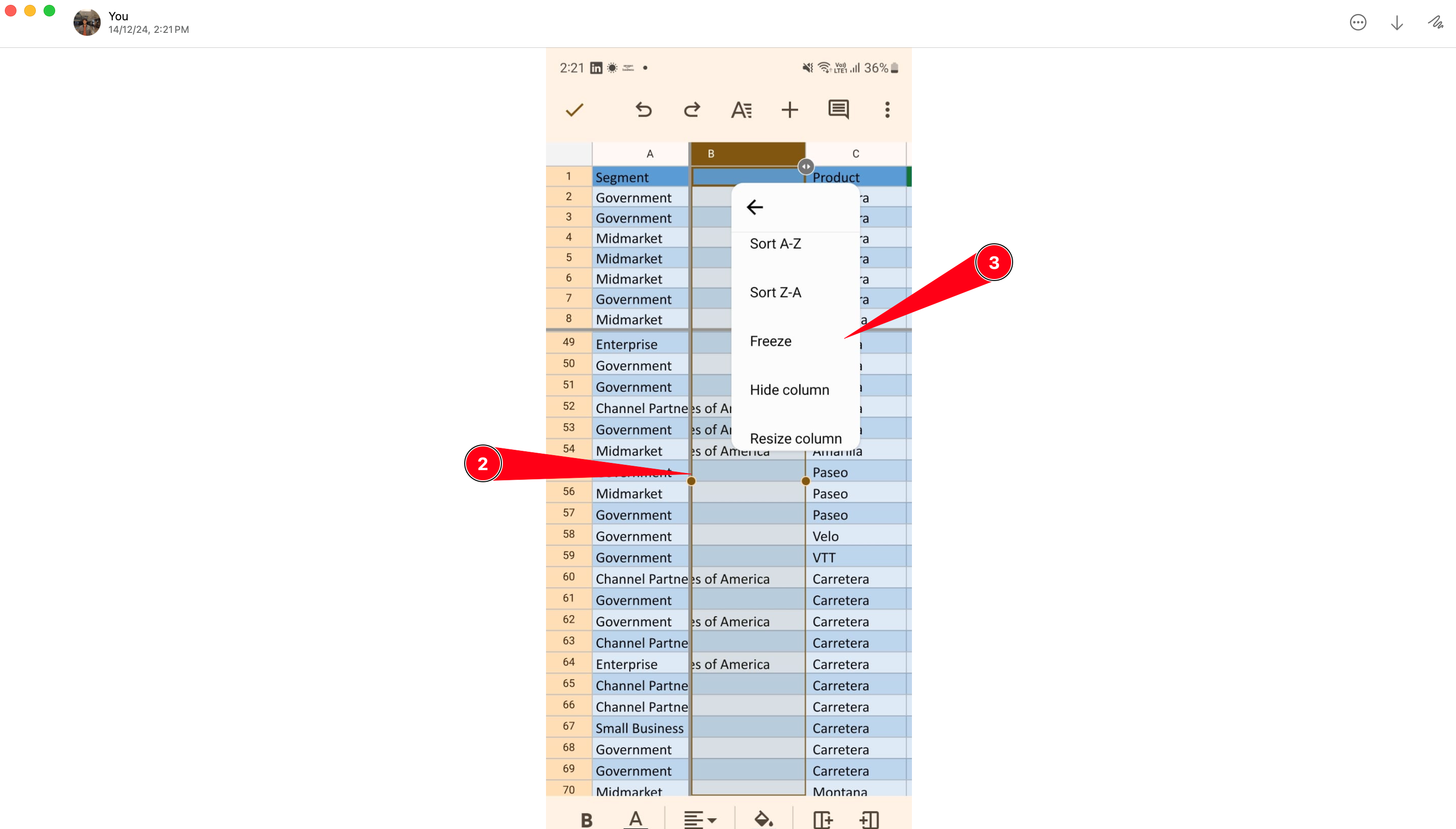
Here’s how:
- Open the Google Sheets App:
- Open the app and select the sheet you want to edit.
- Tap on the Row Number:
- Tap the number of the row you wish to freeze.
- Open the view options:
- Press and hold the cell to open the Freeze or Unfreeze options
- Select Freeze:
- Choose the option to freeze rows, and your selected row will stay visible as you scroll.
Freezing a row that’s not at the top is the same as the steps in the screenshot above. Here’s how you can freeze a middle row in Google Sheets:
- Select the Row:
- Click on the row number of the middle row you want to freeze.
- Drag the Freeze Line:
- Move the thick gray bar from above the top row down to the selected middle row. This freezes all rows above it.
- Verify Freezing:
- Scroll down to check that the selected row and all rows above it remain visible.

Need to freeze columns instead? Follow these steps:
- Select Rows and Columns:
- Identify the columns you want to freeze.
- Go to View Menu:
- Click
View > Freezeand select the appropriate rows and columns.
- Click
For instance, freezing the top row and first column ensures both headers remain visible while navigating the sheet.
- Plan Your Freezing: Decide which rows or columns need to stay visible to improve navigation.
- Adjust as Needed: You can unfreeze rows by selecting
View > Freeze > No rows. - Combine Features: Use the freeze function along with filters to quickly analyze data.
Freezing rows in Google Sheets is an essential feature for managing and navigating large datasets effectively. Whether you’re working on a desktop or using the Google Sheets app, the process is straightforward and highly beneficial for keeping important information accessible. Start freezing rows today to make your spreadsheets more user-friendly and organized!
